Distribution of Prime Numbers
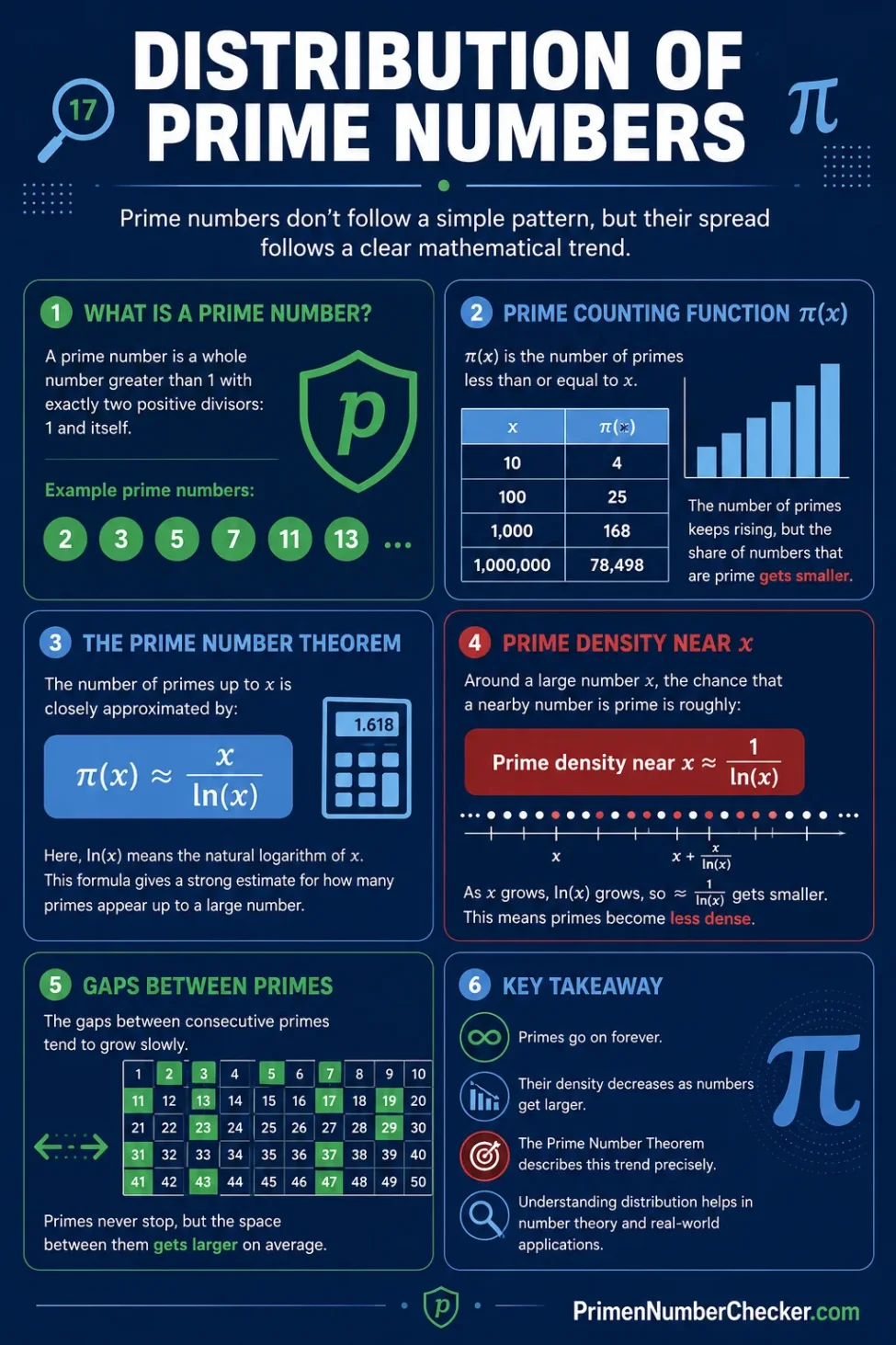
The distribution of prime numbers describes how prime numbers are spread along the number line. Prime numbers do not follow a simple repeating pattern, but they are not random in the same way coin flips are random. Their spread becomes thinner as numbers get larger, and that thinning follows a clear mathematical trend.
The short version is this: near a large number x, about 1 in ln(x) numbers is prime. This idea is closely tied to the Prime Number Theorem, one of the central results in number theory.
If you want to test individual values while studying the pattern, you can use the Prime Number Checker to check whether a number is prime and then connect that result to the wider distribution.
What Does Prime Number Distribution Mean?
The distribution of prime numbers is about placement. It asks where primes appear, how often they appear, and how their frequency changes as numbers grow.
A prime number is a whole number greater than 1 with exactly two positive divisors: 1 and itself. For example, 2, 3, 5, 7, 11, and 13 are prime numbers. Numbers such as 4, 6, 8, 9, and 10 are composite because they have extra divisors.
At first, primes seem common. Between 1 and 10, there are four primes: 2, 3, 5, and 7. But as the number line continues, primes become less frequent. They never stop appearing, yet the space between them tends to grow.
Simple idea
Prime numbers go on forever, but their density decreases. That means primes keep appearing, while the average gap between nearby primes slowly gets larger.
The Prime Counting Function
Mathematicians often study prime distribution using the prime counting function, written as π(x). Here, π(x) does not mean 3.14159. It means the number of primes less than or equal to x.
For example:
| x | π(x) | Meaning |
|---|---|---|
| 10 | 4 | There are 4 primes up to 10. |
| 100 | 25 | There are 25 primes up to 100. |
| 1,000 | 168 | There are 168 primes up to 1,000. |
| 1,000,000 | 78,498 | There are 78,498 primes up to one million. |
This table shows the main pattern. The number of primes keeps rising, but the share of numbers that are prime gets smaller.
The Prime Number Theorem
The Prime Number Theorem gives the main long-range rule for prime distribution. It says that the number of primes up to x is closely approximated by:
π(x) ≈ x / ln(x)
Here, ln(x) means the natural logarithm of x. This formula does not list exact primes. Instead, it gives a strong estimate for how many primes appear up to a large number.
For small numbers, the estimate may feel rough. For large numbers, it becomes much more useful. That is why prime distribution is often studied through patterns over long ranges, not just by looking at a short list of primes.
What the formula means in plain English
The formula x / ln(x) says that primes become less dense as x grows. Around a large number x, the chance that a nearby number is prime is roughly:
Prime density near x ≈ 1 / ln(x)
This is a clean way to understand why primes thin out. For example, ln(100) is about 4.6, so the rough local density near 100 is about 1 in 4.6. Near 1,000,000, ln(x) is about 13.8, so the rough local density is about 1 in 13.8.
Why Do Prime Numbers Thin Out?
As numbers get larger, they have more possible smaller divisors. A large number may be divisible by 3, 5, 7, 11, 13, or many other earlier primes. Each possible divisor creates more chances for a number to be composite.
That does not mean large primes are rare in an absolute sense. There are still infinitely many primes. But among all numbers in a large range, a smaller percentage are prime.
Prime gaps explain the feeling of unevenness
A prime gap is the distance between two consecutive prime numbers. For example, the gap between 11 and 13 is 2. The gap between 23 and 29 is 6.
Prime gaps are not equal. Sometimes primes appear close together, as in twin primes such as 11 and 13. Sometimes there is a longer stretch with no primes. This uneven spacing is one reason prime distribution feels mysterious, even though its average behavior is well understood.
Are Prime Numbers Random?
Prime numbers are not random because each number has a fixed answer: it is either prime or it is not. The number 97 is prime today, tomorrow, and forever. There is no chance involved in that fact.
Still, prime numbers can look irregular when listed in order. Their local pattern is hard to predict by eye. That is why prime distribution has two sides:
- Local behavior: exact placement of nearby primes can look uneven.
- Long-range behavior: prime density follows the smooth trend described by the Prime Number Theorem.
This mix is what makes primes so important in number theory. They are fully determined, yet their placement has a natural-looking irregular rhythm.
Historical Context
The study of prime distribution grew from a simple question: how many primes are there up to a given number? Euclid proved that there are infinitely many primes. Much later, mathematicians such as Gauss and Legendre noticed that the count of primes up to x seemed closely related to logarithms.
The Prime Number Theorem made that observation precise. It showed that π(x) grows like x / ln(x). This changed prime numbers from a list of special integers into a topic with deep structure and measurable density.
Prime Distribution and the Riemann Hypothesis
The Riemann Hypothesis is one of the most famous open problems in mathematics. It is connected to how accurately we can measure the difference between the real prime counting function π(x) and smooth estimates of prime growth.
The Prime Number Theorem gives the main trend. The Riemann Hypothesis is about the fine error pattern around that trend. In simpler terms, it asks how tightly prime numbers follow their expected distribution.
Helpful distinction
The Prime Number Theorem explains the average spread of primes. The Riemann Hypothesis is linked to the smaller waves and errors around that average spread.
Why Prime Distribution Matters
Prime distribution is not only a theoretical topic. It supports several areas of modern mathematics and computing.
Number theory
Prime numbers are the basic indivisible numbers used to study divisibility, factorization, modular arithmetic, and integer structure. Understanding how primes are distributed helps mathematicians study deeper patterns in whole numbers.
Cryptography
Large prime numbers play a role in many encryption systems. These systems do not rely on prime numbers being random. They rely on the difficulty of factoring very large composite numbers made from primes.
Algorithms
Prime distribution affects how prime-search algorithms work. If primes are expected about every ln(x) numbers near x, an algorithm can estimate how far it may need to search before finding a likely prime.
Prime checking tools
A prime checker answers a local question: is this exact number prime? Prime distribution answers a wider question: how common are primes around this size? These ideas work well together. One explains a single number; the other explains the pattern around it.
Common Patterns in Prime Distribution
2 is the only even prime
Every even number greater than 2 is divisible by 2, so it is composite. This immediately removes half of all whole numbers from being prime candidates.
Most primes greater than 3 are near multiples of 6
Every prime greater than 3 has the form 6n − 1 or 6n + 1. This does not mean every number of those forms is prime. For example, 25 is 6 × 4 + 1, but it is not prime. Still, this pattern helps explain why primes appear only in certain residue classes after small divisibility rules are removed.
Prime gaps can grow
There can be long stretches with no primes. For example, the numbers from n! + 2 through n! + n are all composite for any whole number n greater than 1. This shows that prime gaps can become very large.
Primes never end
Even though primes thin out, they do not stop. Euclid’s classic reasoning shows that no final prime can exist. If a list contained every prime, multiplying them together and adding 1 would create a number not divisible by any prime in that list.
How to Read Prime Distribution Without Overthinking It
The best way to understand prime distribution is to separate exact primality from average density.
Exact primality asks whether one number has divisors other than 1 and itself. Average density asks how many primes are expected in a range. These are related, but they are not the same question.
Practical reading
- Use divisibility to decide whether one number is prime.
- Use π(x) to count primes up to a limit.
- Use x / ln(x) to estimate prime count for large x.
- Use 1 / ln(x) to estimate local prime density near x.
FAQ
What is the distribution of prime numbers?
The distribution of prime numbers describes how primes are spread across the number line. Prime numbers become less dense as numbers grow, but they continue forever.
Do prime numbers follow a pattern?
Prime numbers do not follow a simple repeating pattern. However, their average density follows a clear trend described by the Prime Number Theorem.
What is the Prime Number Theorem?
The Prime Number Theorem says that the number of primes up to x is approximately x divided by ln(x). In symbols, π(x) ≈ x / ln(x).
Are prime numbers random?
No. Each number has a fixed prime or composite status. But the local spacing between primes can look irregular, especially when looking at short ranges.
Why do primes become less common?
Larger numbers have more possible smaller divisors, so more of them are composite. This makes the density of primes gradually decrease.