Prime Number Theorem Explained

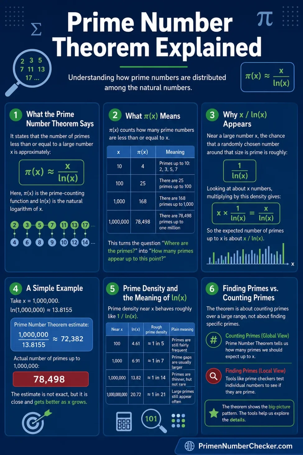
The Prime Number Theorem describes how prime numbers become less common as numbers get larger. More exactly, it says that the number of primes less than or equal to a large number x is approximated by:

π(x) ≈ x / ln(x)

Here, π(x) means the prime-counting function, and ln(x) means the natural logarithm of x. The theorem does not predict the exact location of every prime. It describes the long-term density of primes among the whole numbers.

Near a large number x, roughly 1 out of every ln(x) numbers is prime.

What the Prime Number Theorem Says

Prime numbers look irregular when they are listed one by one:

2, 3, 5, 7, 11, 13, 17, 19, 23, 29…

Sometimes primes appear close together. Sometimes there are long gaps. This makes primes difficult to predict at a local level. When mathematicians count primes over a large range, however, a stable pattern appears.

The Prime Number Theorem states:

The number of primes up to x is asymptotically equal to x divided by the natural logarithm of x.

In symbols:

π(x) ∼ x / ln(x)

The symbol ∼ does not mean that the two expressions are exactly equal. It means that their ratio approaches 1 as x grows.

What π(x) Means

The function π(x) counts how many prime numbers are less than or equal to x. It does not represent the circle constant 3.14159 in this context.

The prime-counting function turns the question “Where are the primes?” into a measurable question: how many primes appear up to this point?

Why x / ln(x) Appears

The expression x / ln(x) appears because primes become thinner in a slow, logarithmic way.

Small ranges contain a relatively high proportion of primes. Between 1 and 10, four numbers are prime. Between 1 and 1,000,000, there are 78,498 primes. The total count rises, but primes form a smaller share of all numbers.

The natural logarithm grows slowly. That growth matches the rate at which prime density decreases. Near a large number x, the rough density of primes is:

1 / ln(x)

Looking across approximately x numbers gives the heuristic calculation:

x × 1 / ln(x) = x / ln(x)

This calculation gives intuition for the formula. The theorem itself requires a proof using methods from analytic number theory.

A Simple Example

Take x = 1,000,000.

The natural logarithm of 1,000,000 is approximately 13.8155. The basic Prime Number Theorem estimate is:

1,000,000 / 13.8155 ≈ 72,382

The actual number of primes up to 1,000,000 is:

78,498

The estimate is not exact, but it shows the correct scale. As x becomes larger, the relative difference between π(x) and x / ln(x) decreases.

Why the Estimate Is Not Exact

Prime numbers are not placed at evenly spaced positions. The theorem describes average behavior across large ranges rather than the exact count at every point.

For smaller values of x, the estimate can have a visible error. The theorem concerns asymptotic behavior: the ratio between the actual count and the estimate approaches 1 as x grows without bound.

Prime Density and the Meaning of ln(x)

The phrase prime density refers to the proportion of numbers in a range that are prime. The Prime Number Theorem says that prime density near x behaves roughly like:

1 / ln(x)

This density estimate applies across ranges, not to the primality of one selected value. You can test an individual number using the Prime Number Checker, while the Prime Number Theorem describes what to expect across many numbers.

The Difference Between Finding Primes and Counting Primes

Two related questions are often confused:

• Is this number prime? This asks about one specific integer.
• How many primes are there up to x? This asks about a range of integers.

A primality test or prime checker answers the first question. The Prime Number Theorem gives an asymptotic answer to the second.

For example, checking whether 999,983 is prime requires a primality test. Asking how many primes exist below 1,000,000 concerns the function π(x).

Exact Results and Statistical Results

Primality is exact: a number either has exactly two positive divisors or it does not. Prime density is statistical: when many integers are considered together, the number of primes follows an asymptotic pattern.

The Prime Number Theorem describes this large-scale pattern. It does not determine the status of one selected integer.

How Accurate Is the Prime Number Theorem?

The estimate x / ln(x) becomes relatively more accurate as x grows, but it is not always the closest practical estimate for smaller ranges.

A related function called the logarithmic integral, usually written as Li(x) or li(x), often gives a closer approximation to π(x). The expression x / ln(x) remains the standard form used to state the Prime Number Theorem.

The theorem is not intended to replace exact prime counting. It describes the asymptotic distribution of primes.

Historical Background

Mathematicians identified the logarithmic pattern before they proved it.

Carl Friedrich Gauss studied tables of primes and observed that their density appeared to decrease according to a logarithmic rule. Adrien-Marie Legendre also proposed formulas for estimating the number of primes below a given number.

The Prime Number Theorem was proved independently in 1896 by Jacques Hadamard and Charles Jean de la Vallée Poussin. Their proofs used complex analysis and properties of the Riemann zeta function.

The result connected the distribution of whole-number primes with the analytic behavior of functions of a complex variable.

Connection to the Riemann Zeta Function

The Prime Number Theorem is closely related to the Riemann zeta function. For complex values s with real part greater than 1, it is defined by:

ζ(s) = 1 + 1/2^s + 1/3^s + 1/4^s + …

Euler showed that the same function can be written as a product over all primes:

ζ(s) = ∏_p 1 / (1 − p^−s)

This is called the Euler product. It reflects the fact that every integer greater than 1 has a unique factorization into primes.

The classical proof of the Prime Number Theorem depends on showing that the zeta function has no zeros on the line Re(s) = 1. This zero-free boundary is enough to establish the asymptotic formula for π(x).

The Critical Strip and the Riemann Hypothesis

The nontrivial zeros of the Riemann zeta function lie in the region:

0 < Re(s) < 1

This region is called the critical strip. The Riemann Hypothesis states that every nontrivial zero in this strip has real part exactly 1/2.

The positions of the zeros are connected to the error between the actual prime-counting function and smooth estimates of prime growth. The Prime Number Theorem gives the main asymptotic term. Information about zeta zeros gives finer control over the error around that term.

Guth–Maynard Result Published in 2026

Larry Guth and James Maynard developed new bounds for the large values of Dirichlet polynomials. These polynomials are used in analytic number theory to study prime numbers and the Riemann zeta function.

Their paper, New Large Value Estimates for Dirichlet Polynomials, was published online by the Annals of Mathematics on March 1, 2026. It appears in Volume 203, Issue 2, on pages 623–675.

The work improves estimates for how often Dirichlet polynomials can take unusually large values. Those estimates lead to stronger results for zeros of the Riemann zeta function and for the distribution of primes in short intervals.

The Improved Zero-Density Estimate

A zero-density estimate limits how many nontrivial zeta zeros can lie to the right of a chosen vertical line inside the critical strip.

If N(σ,T) counts zeros ρ = β + iγ satisfying β ≥ σ and |γ| ≤ T, the Guth–Maynard result gives:

N(σ,T) ≤ T^{30(1−σ)/13+o(1)}

This bound restricts the number of zeros that can occur in certain parts of the critical strip. It does not show that every nontrivial zero lies on the line Re(s) = 1/2.

Primes in Short Intervals

The ordinary Prime Number Theorem counts primes across the full range from 1 to x. A short-interval problem studies a much smaller range beginning near x:

[x, x + h]

When h is much smaller than x, the interval is short relative to its location on the number line. The expected number of primes in such an interval is approximately:

h / ln(x)

Proving that this expected count holds becomes harder as the interval gets shorter. The Guth–Maynard estimates establish the expected asymptotic behavior for intervals of length:

x^17/30+o(1)

Since 17/30 ≈ 0.5667, this interval is far shorter than the full range from 1 to x. The result gives more precise information about prime distribution at a local scale while remaining unconditional.

The Weighted Short-Interval Formula

Analytic number theory often states the short-interval result using the von Mangoldt function, written as Λ(n). This function gives logarithmic weight to prime powers.

The expected asymptotic form is:

∑_x<n≤x+h Λ(n) ∼ h

For interval lengths covered by the Guth–Maynard estimates, the weighted count approaches the expected value. In unweighted terms, this corresponds to approximately h / ln(x) primes in the interval.

What x^17/30+o(1) Means

The term o(1) represents a quantity that tends to zero as x grows. The notation describes an asymptotic threshold rather than one fixed interval length for every value of x.

The result does not claim that every much shorter interval contains a prime or contains exactly the expected number of primes. It identifies a shorter range in which the expected asymptotic distribution can now be proved without assuming the Riemann Hypothesis.

Why the Result Relates to the Prime Number Theorem

The classical Prime Number Theorem gives an average across the interval from 1 to x. The Guth–Maynard result studies whether the same logarithmic density remains visible inside intervals that are small compared with x.

This links three parts of analytic number theory:

• Dirichlet polynomials: finite sums used to approximate and study analytic functions.
• Zero-density estimates: bounds on how many zeta zeros may occur in specified parts of the critical strip.
• Short-interval prime counts: estimates for how primes are distributed near a large value of x.

The result sharpens the known connection between the behavior of zeta zeros and the distribution of primes over shorter ranges.

What the Prime Number Theorem Does Not Say

The Prime Number Theorem does not say that primes are evenly spaced. It does not provide a formula for the next prime, and it does not determine whether a specific number is prime.

It states that over large ranges, the total number of primes follows a logarithmic asymptotic law.

Common Misunderstandings

• It does not list prime numbers. It estimates how many appear up to a limit.
• It does not replace primality testing. A selected number still needs to be tested.
• It does not imply constant prime gaps. Consecutive gaps can vary greatly.
• It does not give exact counts. It gives an asymptotic estimate.
• It does not prove the Riemann Hypothesis. The Prime Number Theorem was proved without resolving that conjecture.
• The 2026 Guth–Maynard result also does not prove the Riemann Hypothesis. It improves zero-density and short-interval estimates.

Prime Gaps and the Theorem

A prime gap is the difference between two consecutive primes. For example, the gap between 11 and 13 is 2, while the gap between 23 and 29 is 6.

The Prime Number Theorem indicates that average prime gaps near x are roughly:

ln(x)

If approximately 1 in every ln(x) numbers near x is prime, the average distance between nearby primes is expected to be about ln(x).

This is only an average. Some gaps are much smaller, including twin-prime gaps of 2. Other gaps are much larger. The theorem does not determine each individual gap.

Why the Prime Number Theorem Matters

The theorem shows that the prime sequence has a measurable average density even though the exact positions of individual primes are uneven.

It also gives practical estimates. If a program searches for a prime near a large value x, the density 1 / ln(x) gives a rough indication of how many candidates may need to be tested.

This applies to computational number theory, random-prime generation, and cryptographic systems that require primes of a chosen size. The theorem does not find those primes, but it estimates how frequently they occur.

Modern primality tests can check large candidates efficiently. The Prime Number Theorem explains why prime searches remain practical even though prime density decreases.

A More Careful Form of the Theorem

The standard form is:

π(x) ∼ x / ln(x)

A more explicit statement is:

As x grows, π(x) divided by x / ln(x) approaches 1.

In limit notation:

lim_x→∞ π(x) / (x / ln(x)) = 1

This limit is the exact mathematical statement behind the usual approximation. It does not require π(x) and x / ln(x) to be identical for any finite value of x.

Why the Limit Form Matters

A reader may calculate x / ln(x), compare it with the exact prime count, and notice that the two numbers differ. That difference does not contradict the theorem.

The theorem describes the ratio of the two quantities as x approaches infinity. It is not an exact counting formula for finite inputs.

What the Prime Number Theorem Means

The theorem can be summarized through four statements:

• Prime numbers never stop.
• They become less frequent as numbers grow.
• Their density decreases at a logarithmic rate.
• The number of primes up to x is asymptotically x / ln(x).

The 2026 Guth–Maynard result adds finer information. It shows that the expected logarithmic distribution can be proved inside shorter intervals of length x^17/30+o(1), using improved estimates connected to zeros of the Riemann zeta function.

FAQ