
A deterministic primality test gives a mathematically certain prime-or-composite result within the domain for which the method is proved. A probabilistic primality test can return a probable-prime result with a controlled chance that a composite number has escaped detection.The distinction is about the guarantee attached to the result, not simply about whether an algorithm is fast or slow. This becomes especially interesting with the Miller–Rabin test: the same underlying test can be probabilistic for unrestricted integers and deterministic when the input is restricted to a proven range and a suitable fixed set of bases is used.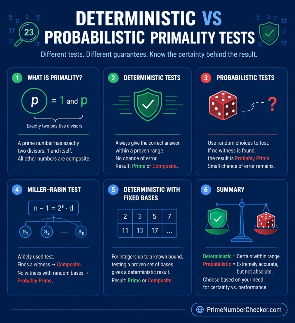
There is a subtle point here. An algorithm that always uses the same bases and therefore produces the same output each time is not automatically a proved deterministic primality test for every integer. Repeatability and mathematical certainty are different properties. A fixed-base method needs a proved validity range before its passing result can be treated as definitive.
If ad mod n = 1 or −1 mod n, the candidate passes that base. Otherwise the value is repeatedly squared, up to the number of stages determined by s. Encountering −1 mod n allows the candidate to pass the round. If the required value never appears, the base is a witness to compositeness.A witness settles the question immediately. The candidate is composite.The opposite result needs more care. Passing one base only means that particular base did not expose the number as composite.
For base 3, 31023 mod 2047 = 1565. That is neither 1 nor 2046. Because s = 1, there is no further squaring stage that could rescue the round. Base 3 therefore proves that 2047 is composite.
This calculator shows the standard independent-round composite-survival bound. It does not calculate the posterior probability that a particular candidate is composite.
For example, a classical smaller-range result uses bases 2, 7, and 61 for integers below 232. The seven-base set shown above extends this style of deterministic Miller–Rabin testing throughout the unsigned 64-bit range.
The central distinction: finding a Miller–Rabin witness proves that a number is composite. Failing to find a witness with randomly chosen bases normally means probably prime. Passing a proven set of bases over a bounded integer range can instead give an exact prime result.
Deterministic and Probabilistic Tests Give Different Guarantees
A primality test asks whether an integer greater than 1 has exactly two positive divisors: 1 and itself. Different algorithms can answer that question with different forms of certainty.| Property | Deterministic test | Probabilistic test |
|---|---|---|
| Prime-side result | Prime | Probably prime |
| Composite result | Composite | Often exact when a witness is found |
| Residual test error | None inside the proved domain | Can be made extremely small |
| Repeated random rounds | Not normally needed | Increase confidence |
| Typical examples | Trial division, AKS, bounded deterministic Miller–Rabin | Random-base Miller–Rabin, Solovay–Strassen |
Why Miller–Rabin Can Be Both Probabilistic and Deterministic
Miller–Rabin is usually introduced as a probabilistic primality test. That description is correct for its general random-base form, but it does not describe every way the test can be used.For an odd candidate n greater than 2, Miller–Rabin begins by writing:n − 1 = 2sd, where d is odd
The test then chooses a base a and computes modular powers. It checks whether the number behaves in a way every prime must behave for that base.1. Decompose n − 1
Write n − 1 as 2sd with odd d.
2. Test a base
Compute ad mod n and, when needed, repeatedly square the result.
3. Look for a witness
If the required prime-like pattern fails, that base proves n is composite.
A Composite Number Can Pass a Miller–Rabin Round
The number 2047 gives a compact example:2047 = 23 × 89
Its factorization proves that it is composite. Yet 2047 passes a Miller–Rabin test using base 2.Since:2047 − 1 = 2046 = 2 × 10²³
we have s = 1 and d = 1023. For base 2:21023 mod 2047 = 1
That is an allowed Miller–Rabin value, so 2047 passes the base-2 round even though it is not prime. In this setting, 2047 is a strong pseudoprime to base 2.Base 2: Pass2047 behaves like a prime for this Miller–Rabin base.
Base 3: CompositeBase 3 exposes the failure, so the test can stop.
Passing one base is not a primality proof. It says that the chosen base did not find evidence of compositeness. Additional independent bases reduce the chance that a composite number keeps escaping detection.
The Miller–Rabin Error Bound
For an odd composite integer, at least three quarters of the possible Miller–Rabin bases expose its compositeness. Equivalently, at most one quarter can act as strong liars for that composite number.If bases are chosen independently and uniformly in the standard random-base setting, the usual worst-case survival bound after k rounds is:P(composite survives k rounds) ≤ 4−k = 2−2k
| Independent rounds | Bound | Maximum survival probability |
|---|---|---|
| 1 | 1 / 4 | 25% |
| 2 | 1 / 16 | 6.25% |
| 5 | 1 / 1,024 | 0.09765625% |
| 10 | 1 / 1,048,576 | 0.000095367431640625% |
| 20 | 1 / 1,099,511,627,776 | about 9.09 × 10⁻¹¹% |
| 32 | 1 / 264 | about 5.42 × 10⁻¹⁸% |
What 4−k does not mean
The formula is often described too loosely. It is not automatically the probability that a particular candidate is composite after it passes k rounds.Those are different probability questions. The 4−k result bounds the chance that a composite input survives independently selected Miller–Rabin rounds. The probability that a randomly generated candidate is composite after passing also depends on how candidates were selected and on the prior distribution of primes and composites.NIST FIPS 186-5 makes this distinction when discussing Miller–Rabin testing for prime generation. The standard treats the probability that a composite survives testing separately from the probability that a candidate surviving the testing process is composite.Precision matters: 4−k is best presented as a worst-case composite-survival bound under the independent random-base assumptions, not as a universal posterior probability that the tested number is composite.
Miller–Rabin Error Bound Calculator
Choose the number of independent random-base rounds to see the standard 4−k composite-survival bound.Rounds
10
Exact form
4^-10 = 2^-20
Decimal bound
9.5367431640625e-7
Equivalent frequency
1 in 1,048,576
The 64-Bit Range Changes the Result
Miller–Rabin becomes especially useful when the allowed input range is known in advance. Instead of choosing random bases indefinitely, it is possible to use a fixed collection of bases that has been proved to detect every composite number below a stated bound.For integers below 264, the following seven Miller–Rabin bases form such a set:2
325
9,375
28,178
450,775
9,780,504
1,795,265,022
If an integer n < 264 passes the required strong probable-prime tests for this proved base set, the result is not merely “probably prime.” Within that range, the combined test is deterministic.Proved 64-bit range
This is why the statement “Miller–Rabin is probabilistic” needs context. The general random-base algorithm is probabilistic. A bounded version using bases proved for the entire permitted range can be exact.For an individual integer in the supported machine-size range, the Prime Number Checker provides the prime-or-composite result directly. The bounded-range idea explains how fast computational primality tests can return certainty without trying every possible divisor.0
264 − 1 = 18,446,744,073,709,551,615
Every possible input in this bounded range is covered by the proved base-set guarantee when the test is implemented correctly.How Fixed Bases Turn a Probable-Prime Test Into an Exact Test
The transformation is not caused merely by replacing random bases with fixed ones. The mathematical guarantee comes from the fact that the selected bases collectively catch every composite integer in the stated range.Suppose a candidate survives base 2. Some composite numbers do. It then faces another base selected specifically because the combined base set has no composite survivor over the bounded domain. Testing continues until either a witness is found or the complete proved set has been passed.Random bases
Unrestricted integers normally lead to a probabilistic guarantee.
Fixed bases without a proved bound
Reproducible results do not by themselves prove primality.
Fixed bases with a proved bound
The test becomes deterministic inside that range.
A bound cannot be discarded. A base set proved for n < 264 should not be presented as a deterministic test for arbitrary larger integers. Beyond its proved range, the same guarantee no longer follows.
Why Fermat Testing Is Weaker Than Miller–Rabin
Fermat’s little theorem gives a tempting primality condition. If p is prime and a is not divisible by p, then:ap−1 ≡ 1 (mod p)
This produces a simple probable-prime test: choose a base and check the congruence. Failure proves compositeness. Passing, however, can be misleading.Some composite integers are Fermat pseudoprimes for particular bases. Carmichael numbers go further: they satisfy the Fermat congruence for every base that is coprime to the number. Repeating an ordinary Fermat test with more such bases therefore does not give the same type of protection as repeated Miller–Rabin rounds.Miller–Rabin examines the sequence of square roots that appears when n − 1 is written as 2sd. This stronger condition exposes many composites that pass the simpler Fermat test.| Test | What a failure means | Main limitation of a pass |
|---|---|---|
| Fermat | Composite | Pseudoprimes and Carmichael numbers can imitate prime behavior |
| Miller–Rabin | Composite | A strong pseudoprime may pass a particular base |
| Repeated random-base Miller–Rabin | Composite if any round finds a witness | Residual composite-survival bound decreases as 4−k |
“Probably Prime” Does Not Mean “Maybe Prime”
The phrase probably prime can sound weaker than it is. It is a technical result label, not an informal guess.Miller–Rabin has a one-sided error structure in its standard probabilistic form. A genuine prime passes every valid base. A composite may occasionally imitate the expected behavior for a chosen base.The two outcomes are therefore not symmetric:Witness found → Composite.
The witness is mathematical evidence that the number is not prime.No witness found → Passed this round.
Another independent base can test the candidate again.All bases in a proved bounded set passed → Prime within that range.
The range-specific theorem removes the residual probable-prime uncertainty.
This distinction also explains why software should be careful with result wording. A general probabilistic test should not silently turn “probably prime” into “proved prime” unless another theorem, bounded-domain result, or primality proof justifies that stronger label.Deterministic Does Not Mean Faster
Certainty and speed are separate properties. A test can be deterministic and inefficient for large inputs, or probabilistic and extremely fast.Trial division
Trial division is deterministic. To prove that n is prime, it is enough to rule out divisors through √n. The reasoning is exact: if n = ab, both factors cannot be greater than √n.The problem is scale. The numerical size of √n grows far faster than the number of bits needed to write n. Straight trial division is therefore useful for small integers but becomes unattractive for very large candidates.AKS
The AKS primality test, introduced by Manindra Agrawal, Neeraj Kayal, and Nitin Saxena, established that primality can be decided by an unconditional deterministic polynomial-time algorithm.That result settled a long-standing complexity-theory question. It did not make AKS the default practical test for every large integer.Polynomial-time describes how running time scales with input length. It does not say that the implementation will beat methods with lower practical overhead on the sizes computers routinely process. Modular-exponentiation methods such as Miller–Rabin are much better suited to many practical primality-testing workloads.Bounded deterministic Miller–Rabin
Machine-size integers create a useful middle case. The domain contains only a finite range of values, and proved base sets can cover that entire range. This gives a test that is both fast in practice and deterministic over its stated domain.| Method | Guarantee | Best fit |
|---|---|---|
| Trial division | Deterministic | Small integers and direct mathematical verification |
| Fermat test | Probable-prime test | Simple illustration of pseudoprime behavior |
| Random-base Miller–Rabin | Probabilistic with a controlled one-sided error | Large unrestricted candidates |
| Bounded fixed-base Miller–Rabin | Deterministic inside its proved range | 32-bit and 64-bit integer testing |
| AKS | Deterministic polynomial time | Theoretical study of primality complexity |
Why AKS Did Not Replace Miller–Rabin
AKS answered a theoretical question: can primality be decided deterministically in polynomial time without relying on an unproved conjecture? Yes.Software has a different question: which correct method gives the desired guarantee efficiently for the actual input size?For a bounded 64-bit integer, a small number of modular exponentiation tests can settle primality exactly. For much larger candidates, repeated Miller–Rabin testing can make composite survival extraordinarily unlikely while remaining fast. AKS offers deterministic polynomial-time behavior, but that alone does not make it the fastest practical choice.This is a useful reminder that algorithm categories do not form a simple ranking. Deterministic describes certainty. Polynomial time describes asymptotic growth. Fast in practice describes actual computation on relevant inputs. They answer different questions.Probabilistic Primality Testing in Cryptographic Standards
Probabilistic primality testing is not merely an educational shortcut. NIST FIPS 186-5 includes Miller–Rabin probabilistic primality testing in procedures associated with RSA prime generation.The terminology used there is revealing: the ordinary Miller–Rabin procedure can return PROBABLY PRIME or COMPOSITE. The number of rounds is chosen according to the required testing conditions rather than pretending that one random round proves primality.That usage reflects the practical value of controllable error. When the mathematical bound is understood and the procedure is designed correctly, a probabilistic test can provide an extremely high level of confidence without the cost of a general deterministic proof method.Primality Testing and Primality Proving Are Different Goals
A program that decides whether a number is prime and a method that produces a compact proof another program can independently verify are related, but they are not identical tasks.Three levels are useful to separate:- Composite detection: find evidence such as a divisor or Miller–Rabin witness that proves the candidate is composite.
- Probable-prime testing: subject the candidate to tests whose failure detects compositeness and whose repeated success gives very high confidence.
- Primality proving: establish primality with a proof or certificate whose validity does not depend on a residual test-error probability.
Choosing a Test by the Guarantee You Need
| Situation | Suitable approach | Reason |
|---|---|---|
| Small integer checked by hand | Trial division through √n | Simple, transparent, and exact |
| Many integers inside a proved 32-bit or 64-bit range | Bounded deterministic Miller–Rabin | Combines exact results with efficient modular arithmetic |
| Arbitrarily large candidate | Repeated Miller–Rabin | Fast testing with an error bound that falls exponentially with the number of rounds |
| Study of deterministic polynomial-time primality | AKS | Provides an unconditional polynomial-time result |
| An independently verifiable primality proof is required | Primality-proving method | A probable-prime result and a verifiable proof serve different purposes |
The Proven Domain Is Part of the Algorithm
When comparing primality tests, the algorithm name alone is not enough. The guarantee depends on the exact way the test is used.For Miller–Rabin, four questions settle most of the ambiguity:- Is the input range bounded? A condition such as n < 264 can allow a deterministic base set.
- Are the bases random or fixed? Random independent bases support a probabilistic error bound; fixed bases can support deterministic testing when a theorem covers the range.
- What does a passing result mean? It may mean “passed this base,” “probably prime,” or “prime within the proved domain.”
- What has actually been proved? A base set that is exact below one bound should not be extended to larger integers without another mathematical result.